

This blog summarizes learnings from Systems Performance by Brendan Gregg that covers concepts, tools, and performance tuning for operating systems and applications.
1. Introduction
This chapter introduces Systems Performance including all major software and hardware components with goals to improve the end-user experience by reducing latency and computing cost. The author describes challenges for performance engineering such as subjectivity without clear goals, complexity that requires holistic approach, multiple causes, and multiple performance issues. The author defines key concepts for performance such as:
Latency: measurement of time spent waiting and it allows maximum speedup to be estimated.
Observability: refers to understanding a system through observation and includes that use counters, profiling, and tracing. This relies on counters, statistics, and metrics, which can be used to trigger alerts by the monitoring software. The profiling performs sampling to paint the picture of target. Tracing is event-based recording, where event data is captured and saved for later analysis using static instrumentation or dynamic instrumentation. The latest dynamic tools use BPF (Berkley Packet Filter) to build dynamic tracing, which is also referred as eBPF.
Experimentation tools: benchmark tools that test a specific component, e.g. following example performs a TCP network throughput:
iperf -c 192.168.1.101 -i 1 -t 10The chapter also describes common Linux tools for analysis such as:
dmesg -T | tail
vmstat -SM 1
mpstat -P ALL 1
pidstat 1
iostat -sxz 1
free -m
sar -n DEV 1
sar -n TCP,ETCP 1
2. Methodologies
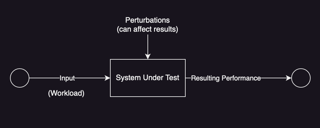
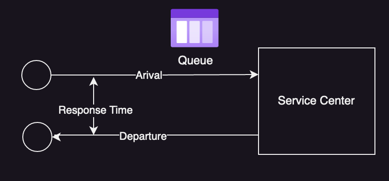
This chapter introduces common performance concepts such as IOPS, throughput, response-time, latency, utilization, saturation, bottleneck, workload, and cache. It defines following models of system performance like System under Test and Queuing System shown below:
The chapter continues with defining concepts such as latency, time-scales, trade-offs, tuning efforts, load vs architecture, scalability, and metrics. It defines utilization based on time as:
U = B / T
where U = utilization, B = total-busy-time, T = observation period
and in terms of capacity, e.g.
U = % used capacityThe chapter defines saturation as the degree to which a resource has queued work it cannot service and defines caching considerations to improve performance such as hit ratio, cold-cache, warm-cache, and hot-cache.
The author then describes analysis perspectives and defines resource analysis that begins with analysis of the system resources for investigating performance issues and capacity planning, and workload analysis that examines the performance of application for identifying and confirming latency issues. Next, author describes following methodologies for analysis:
Streetlight Anti-Method: It is an absence of a deliberate methodology and user analyzes a familiar tool but can be a hit or miss.
Random Change Anti-Method: In this approach, user randomly guesses where the problems may be and then changes things until it goes away.
Blame-Someone-Else Anti-Method: In this approach, user blames someone else and redirects the issue to another team.
Ad Hoc Checklist Method: It’s a common methodology where a user uses an ad hoc list built from recent experience.
Problem Statement: It defines the problem statement based on if there has been a performance issue; what was changed recently; who are being affected; etc.
Scientific Method: This approach is summarized as: Question -> Hypothesis -> Prediction -> Test -> Analysis.
Diagnostic Cycle: This is defined as hypothesis -> instrumentation -> data -> hypothesis.
Tools Method: This method lists available performance tools; gather metrics from each tool; and then interpret the metrics collected.
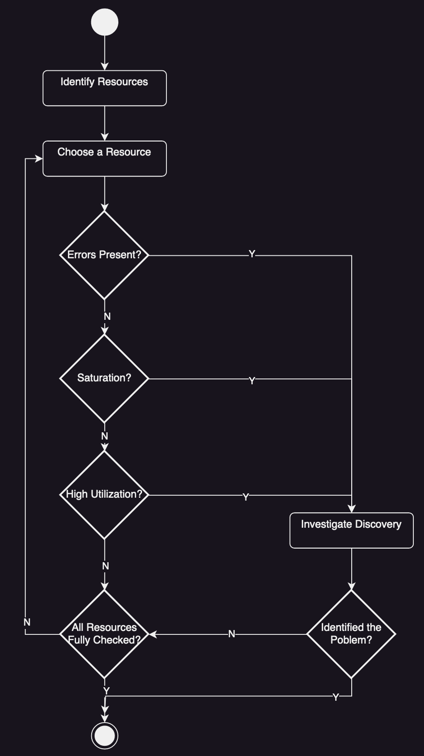
Utilization, Saturation, and Errors (USE) Method: This method focuses on system resources and checks utilization, saturation and errors for each resource.
RED Method: This approach checks request rate, errors, and duration for every service.
Workload Characteristics: This approach answers questions about Who is causing the load; why is the load being called; what are the load characteristics?
Drill-Down Analysis: This approach defines three-stage drill-down analysis methodology for system resource: Monitoring, Identification, Analysis.
Latency Analysis: This approach examines the time taken to complete an operation and then breaks it into smaller components, continuing to subdivide the components.
Method R: This methodology developed for Oracle database that focuses on finding the origin of latency.
Modeling
The chapter then defines analytical modeling of a system using following techniques:
Enterprise vs Cloud
Visual Identification uses graphs to identify patterns for linear scalability, contention, coherence (propagation of changes), knee-point (where performance stops scaling linearly), scalability ceiling.
Admdahl’s Law of Scalability describes content for the serial resource:
C(N) = N / (1 + a(N - 1))
where C(N) is relative capacity, N is scaling dimension such as number of CPU, and a is degree of seriality.
Universal Scalability Law is described as:
C(N) = N / (1 + a(N - 1) + bN(N - 1))
where b is the coherence parameter and when b = 0, it becomes Amdahl's Law
Queuing Theory describes Little’s Law as:
L = lambda * W
where L is average number of requests in the system, lambda is average arrival rate, and W is average request time.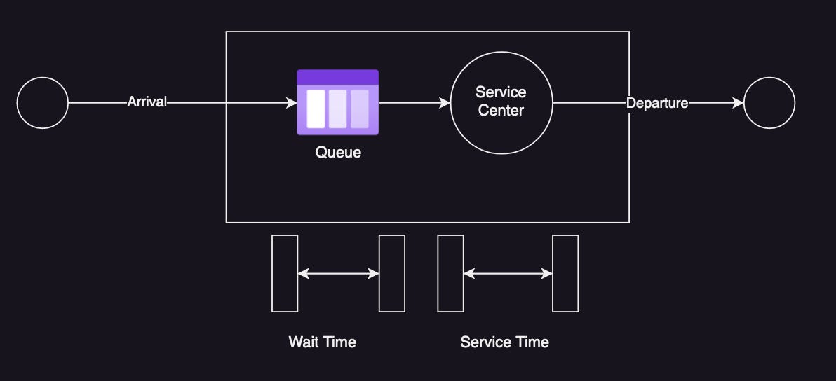
Capacity Planning
This section describes Capacity Planning for examining how system will handle load and will scale as load scales. It searches for a resource that will become the bottleneck under load including hardware and software components. It then applies factor analysis to determine what factors to change to achieve the desired performance.
Statistics
This section reviews how to use statistics for analysis such as:
Quantifying Performance Gains: using observation-based and experimentation-based techniques to compare performance improvements.
Averages: including geometric-mean (nth root of multiplied values), harmonic-mean (count of values divided by sum of their reciprocals), average over time, decayed average (recent time weighed more).
Standard Deviation, Percentile, Median
Coefficient of Variations
Multimodal Distribution
Monitoring
Monitoring records performance statistics over time for comparison and identification using various time-based patterns such as hourly, daily, weekly, and yearly.
Visualization
This section examines various visualization graphs such as line-chart, scatter-plots, heat-maps, timeline-charts, and surface plot.
3. Operating Systems
This chapter examines operating system and kernel for system performance analysis and defines concepts such as:
Background
Kernel
Kernel is the core of operating system and though Linux and BSED have a monolithic kernel but other kernel models include micokernels, unikernels and hybrid kernels. In addition, new Linux versions include extended BPF for enabling secure kernel-mode applications.
Kernel and User Modes
The kernel runs in a kernel mode to access devices and execution of the privileged instructions. User applications run in a user mode where they can request privileged operations using system calls such as ioctl, mmap, brk, and futex.
Interrupts
An interrupt is a single to the processor that some event has occurred that needs processing, and interrupts the current execution of the processor and runs interrupt service routine to handle the event. The interrupts can be asynchronous for handling interrupt service requests (IRQ) from hardware devices or synchronous generated by software instructions such as traps, exceptions, and faults.
Clocks and Idle
In old kernel implementations, tick latency and tick overhead caused some performance issues but modern implementations have moved much functionality out of the clock routine to on-demand interrupts to create tickless kernel for improving power efficiency.
Processes
A process is an environment for executing a user-level program and consists of memory address space, file descriptors, thread stacks, and registers. A process contains one or more threads, where each thread has a stack, registers and an instruction pointer (PC). Processes are normally created using fork system call that wraps around clone and exec/execve system call.
Stack
A stack is a memory storage area for temporary data, organized as last-in, first-out (FIFO) list. It is used to store the return address when calling a function and passing parameters to function, which is also referred as a stack frame. The call path can be seen by examining saved return addresses across all the stack frames, which is called stack trace or stack back trace. While executing a system call, a process thread has two stacks: a user-level stack and a kernel-level stack.
Virtual Memory
Virtual memory is an abstraction of main memory, providing processes and the kernel with their own private view of main memory. It supports multitasking of threads and over-subscription of main memory. The kernel manages memory using process-swapping and paging schemes.
Schedulers
The scheduler schedules processes on processors by dividing CPU time among the active processes and threads. The scheduler tracks all threads in the read-to-run state in run priority-queues where process priority can be modified to improve performance of the workload. Workloads are categorized as either CPU-bound or I/O bound and scheduler may decrease the priority of CPU-bound processes to allow I/O-bound workloads to run sooner.
File Systems
File systems are an organization of data as files and directories. The virtual file system (VFS) abstracts file system types so that multiple file systems may coexist.
Kernels
This section discusses Unix-like kernel implementations with a focus on performance such as Unix, BSD, and Solaris. In the context of Linux, it describes systemd, which is a commonly used service manager to replace original UNIX init system and extended BPF that can be used for networking, observability, and security. BPF programs run in kernel model and are configured to run on events like USDT probes, kprobes, uprobes, and perf_events.
4. Observability Tools
This chapter identifies static performance and crises tools including their overhead like counters, profiling, and tracing.
Tools Coverage
This section describes static performance tools like sysctl, dmesg, lsblk, mdadm, ldd, tc, etc., and crisis tools like vmstat, ps, dmesg, lscpu, iostat, mpstat, pidstat, sar, and more.
Tools Type
The observability tool can categorized as a system-wide, per-process observability or counters/events based, e.g. top shows system-wide summary; ps, pmap are maintained per-process; and profilers/tracers are event-based tools. Kernel maintains various counters that are incremented when events occur such as network packets received, disk I/O, etc. Profiling collects a set of samples such as CPU usage at fixed-rate or based on untimed hardware events, e.g., perf, profile are system-wide profilers, and gprof and cachegrind are per-process profilers. Tracing instruments occurrence of an event, and can store event-based details for later analysis. Examples of system-wide tracing tools include tcpdump, biosnoop, execsnoop, perf, ftrace and bpftrace, and examples of per-process tracing tools include strace and gdb. Monitoring records statistics continuously for later analysis, e.g. sar, prometheus, collectd are common tools for monitoring.
Observability Sources
The main sources of system performance include /proc and /sys. The /proc is a file system for kernel statistics and is created dynamically by the kernel. For example, ls -F /proc/123 lists per-process statistics for process with PID 123 like limits, maps, sched, smaps, stat, status, cgroup and task. Similarly, ls -Fd /proc/[a-z]* lists system-wide statistics like cpuinfo, diskstats, loadavg, meminfo, schedstats, and zoneinfo. The /sys was originally designed for device-driver statistics but has been extended for other types of statistics, e.g. find /sys/devices/system/cpu/cpu0 -type f provides information about CPU caches. Tracepoints are Linux kernel event source based on static instrumentation and provide insight into kernel behavior. For example, perf list tracepoint lists available tracepoints and perf trace -e block:block_rq_issue traces events. Tracing tools can also use tracepoints, e.g., strace -e openat ~/iosnoop and strace -e perf_event_open ~/biosnoop. A kernel event source based on dynamic instrumentation includes kprobes that can trace entry to functions and instructions, e.g. bpftrace -e 'kprobe:do_nanosleep { printf("sleep %s\n", comm); }'. A user-space event-source for dynamic instrumentation includes uprobes, e.g., bpftrace -l 'uprob:/bin/bash:*'. User-level statically-defined tracing (UsDT) is the user-space version of tracepoint and some libraries/apps have added USDt probes, e.g., bpftrace -lv 'usdt:/openjdk/libjvm.so:*'. Hardware counters (PMC) are used for observing activity by devices, e.g. perf stat gzip words instruments the architectural PMCs.
Sar
Sar is a key monitoring tool that is provided via the sysstat package, e.g., sar -u -n TCP,ETCP reports CPU and TCP statistics.
5. Applications
This chapter describes performance tuning objectives, application basics, fundamentals for application performance, and strategies for application performance analysis.
Application Basics
This section defines performance goals including lowering latency, increasing throughput, improving resource utilization, and lowering computing costs. Some companies use a target application performance index (ApDex) as an objective and as a metric to monitor:
Apdex = (satisfactory + 0.5 x tolerable + 0 x frustrating) / total-eventsApplication Performance Techniques
This section describes common techniques for improving application performance such as increasing I/O size to improve throughput, caching results of commonly performed operations, using ring buffer for continuous transfer between components, and using event notifications instead of polling. This section describes concurrency for loading multiple runnable programs and their execution that may overlap, and recommends parallelism via multiple processes or threads to take advantage of multiprocessor systems. These multiprocess or multithreaded applications use CPU scheduler with the cost of context-switch overhead. Alternatively, use-mode applications may implement their own scheduling mechanisms like fibers (lightweight threads), co-routines (more lightweight than fiber, e.g. Goroutine in Golang), and event-based concurrency (as in Node.js). The common models of user-mode multithreaded programming are: using service thread-pool, CPU thread-pool, and staged event-driven architecture (SEDA). In order to protect integrity of shared memory space when accessing from multiple threads, applications can use mutex, spin locks, RW locks, and semaphores. The implementation of these synchronization primitives may use fastpath (using cmpxchg to set owner), midpath (optimistic spinning), slowpath (blocks and deschedules thread), or read-copy-update (RCU) mechanisms based on the concurrency use-cases. In order to avoid the cost of creation and destruction of mutex-locks, the implementations may use hashtable to store a set of mutex locks instead of using a global mutex lock for all data structures or a mutex lock for every data structure. Further, non-blocking allows issuing I/O operations asynchronously without blocking the thread using O_ASYNC flag in open, io_submit, sendfile and io_uring_enter.
Programming Languages
This section describes compiled languages, compiler optimization flags, interpreted languages, virtual machines, and garbage collection.
Methodology
This section describes methodologies for application analysis and tuning using:
CPU profiling and visualizing via CPU flame graphs.
off-CPU analysis using sampling, scheduler tracing, and application instrumentation, which may be difficult to interpret due to wait time in the flame graphs so zooming or kernel-filtering may be required.
Syscall analysis can be instrumented to study resource based performance issues where the target for syscall analysis include new process tracing, I/O profiling, and kernel time analysis.
USE method
Thread state analysis like user, kernel, runnable, swapping, disk I/O, net I/O, sleeping, lock, idle.
Lock analysis
Static performance tuning
Distributed tracing
Observability Tools
This section introduces application performance observability tools:
perf is standard Linux profiler with many uses such as:
CPU Profiling:
perf record -F 49 -a -g -- sleep 30&&per script --header > out.stackCPU Flagme Graphs:
./stackcollapse-perf.pl < out.stacks | ./flamgraph.ol --hash > out.svgSyscall Tracing:
perf trace -p $(pgrep mysqld)Kernel Time Analysis:
perf trace -s -p $(pgrep mysqld)
porfile is timer-based CPU profiler from BCC, e.g.,
profile -F 49 10
offcputime and bpftrace to summarize time spent by thrads blocked and off-CPU, e.g.,
offcputime 5
strace is the Linux system call tracer
strace -ttt -T -p 123
execsnoop traces new process execution system-wide.
syscount to count system call system wide.
bpftrace is a BPF-based tracer for high-level programming languages, e.g.,
bpftrace -e 't:syscalls:sys_enter_kill { time("%H:%M:%S "); }'
6. CPU
This chapter provides basis for CPU analysis such as:
Models
This section describes CPU architecture and memory caches like CPU registers, L1, L2 and L3. It then describes run-queue that queue software threads that are ready to run and time spent waiting on CPU run-queue is called run-queue latency or dispatcher-queue latency.
Concepts
This section describes concepts regarding CPU performance including:
Clock Rate: Each CPU instruction may take one or more cycles of the clock to execute.
Instructions: CPU execute instructions chosen from their instruction set.
Instruction Pipeline: This allows multiple instructions in parallel by executing different components of different instructions at the same time. Modern processors may implement branch prediction to perform out-of-order execution of the pipeline.
Instruction Width: Superscalar CPU architecture allows more instructions can make progress with each clock cycle based on the width of instruction.
SMT: Simultaneous multithreading makes use of a superscalar architecture and hardware multi-threading support to improve parallelism.
IPC, CP: Instructions per cycle ((IPC) describe how CPU is spending its clock cycles.
Utilization: CPU utilization is measured by the time a CPU instance is busy performing work during an interval.
User Time/Kernel Time: The CPU time spent executing user-level software is called user time, and kernel-time software is kernel time.
Saturation: A CPU at 100% utilization is saturated, and threads will encounter scheduler lateny as they wait to run on CPU.
Priority Inversion: It occurs when a lower-priority threshold holds a resource and blocks a high priority thread from running.
Multiprocess, Multithreading: Multithreading is generally considered superior.
Architecture
This section describes CPU architecture and implementation:
Hardware
CPU hardware include processor and its subsystems:
Processor: The processor components include P-cache (prefetch-cache), W-cache (write-cache), Clock, Timestamp counter, Microcode ROM, Temperature sensor, and network interfaces.
P-States and C-States: The advanced configuration and power interface (ACPI) defines P-states, which provides different levels of performance during execution, and C-states, which provides different idle states for when execution is halted, saving power.
CPU caches: This include levels of caches like level-1 instruction cache, level-1 data cache, translation lookaside buffer (TLB), level-2 cache, and level-3 cache. Multiple levels of cache are used to deliver the optimum configuration of size and latency.
Associativity: It describes constraint for locating new entries like full-associative (e.g. LRU), direct-mapped where each entry has only one valid location in cache, set-associative where a subset of the cache is identified by mapping, e.g., four-way associative maps an address to four possible location.
Cache Line: Cache line size is a range of bytes that are stored and transferred as a unit.
Cache Coherence: Cache coherence ensures that CPUs are always accessing the correct state of memory.
MMU: The memory management unit (MMU) is responsible for virtual-to-physical address translation.
Hardware Counters (PMC): PMCs are processor registers implemented in hardware and include CPU cycles, CPU instructions, Level 1, 2, 3 cache accesses, floating-point unit, memory I/O, and resource I/O.
GPU: GPU support graphical displays.
Software: Kernel software include scheduler that performs time-sharing, preemption, and load balancing. The scheduler uses scheduling classes to manage the behavior of runnable threads like priorities and scheduling policies. The scheduling classes for Linux kernels include RT (fixed and high-priorities for real-time workloads), O(1) for reduced latency, CFS (Completely fair scheduling), Idle, and Deadline. Scheduler policies include RR (round-robin), FIFO, NORMAL, BATCH, IDLE, and DEADLINE.
Methodology
This section describes various methodologies for CPU analysis and tuning such as:
Tools Method: iterate over available tools like uptime, vmstat, mpstat, perf/profile, showboost/turboost, and dmesg.
USE Method: It checks for utilization, saturation, and errors for each CPU.
Workload Charcterization like CPU load average, user-time to system-time ratio, syscall rate, voluntary context switch rate, and interrupt rate.
Profiling: CPU profiler can be performed by time-based sampling or function tracing.
Cycle Analysis: Using performance monitor counter ((PMC) to understand CPU utilization at the cycle level.
Performance Monitoring: identifies active issues and patterns over time using metrics for CPU like utilization and saturation.
Static Performance Tuning
Priority Tuning
CPU Binding
Observability Tools
This section introduces CPU performance observability tools such as:
uptime
load average – exponentially damped moving average for load including current resource usage plus queued requests (saturation).
pressure stall information (PSI)
vmstat, e.g.
vmstat 1mpstat, e.g.
mpstat -P ALL 1sar
ps
top
pidstat
time, ptime
turbostat
showboost
pmcash
tlbstat
perf, e.g.,
perf record -F 99 command,perf stat gzip ubuntu.iso, and perf stat -a -- sleep 10profile
cpudist, e.g.,
cpudist 10 1runqlat, e.g.,
runqlat 10 1runqlen, e.g.,
runqlen 10 1softirqs, e.g.,
softirqs 10 1hardirqs, e.g.,
hardirqs 10 1bpftrace, e.g.,
bpftrace -l 'tracepoint:sched:*'
Visualization
This section introduces CPU utilization heat maps, CPU subsecond-offset heat maps, flame graphs, and FlameScope.
Tuning
The tuning may use scheduling priority, power stats, and CPU binding.
7. Memory
This chapter provides basis for memory analysis including background information on key concepts and architecture of hardware and software memory.
Concepts
Virtual Memory
Virtual memory is an abstraction that provides each process its own private address space. The process address space is mapped by the virtual memory subsystem to main memory and the physical swap device.
Paging
Paging is the movement of pages in and out of main memory. File system paging (good paging) is caused by the reading and writing of pages in memory-mapped files. Anonymous paging (bad paging) involves data that is private to process: the process heap and stacks.
Demand Paging
Demand paging map pages of virtual memory to physical memory on demand and defers the CPU overhead of creating the mapping until they are needed.
Utilization and Saturation
If demands for the memory exceeds the amount of main memory, main memory becomes saturated and operating system may employ paging or OOM killer to free it.
Architecture
This section introduces memory architecture:
Hardware Main Memory
The common type of the main memory is dynamic random-access memory (DRAM) and column address strobe (CAS) latency for DDR4 is around 10-20ns. The main memory architecture can be uniform memory access (UMA) or non-uniform memory access (NUMA). The main memory may use a shared system-bus to connect a single or multiprocessors, directly attached memory, or interconnected memory bus. The MMU (memory management unit) translates virtual addresses to physical addresses for each page and offset within a page. The MMU uses a TLB (translation lookaside buffer) as a first-level cache for addresses in the page tables.
Software
The kernel tracks free memory in free list of pages that are available for immediate allocation. The kernel may use swapping, reap any memory that can be freed, or use OOM killer to free memory when memory is low.
Process Virtual Address Space
The process virtual address space is a range of virtual pages that are mapped to physical pages and addresses are split into segments like executable text, executable data, heap, and stack. There are a variety of user- and kernel-level allocators for memory with simple APIs (malloc/free), effcient memory usage, performance, and observability.
Methodology
This section describes various methodlogies for memory analysis:
Tools Method: involves checking page scanning, pressure stall information (PSI), swapping, vmstat, OOM killer, and perf.
USE Method: utilization of memory, the degree of page scanning, swapping, OOM killer, and hardware errors.
Characterizing usage
Performance monitoring
Leak detection
Static performance tuning
Observability Tools
This section includes memory observability tools including:
vmstat
PSI, e.g.,
cat /proc/pressure/memoryswapon
sar
slabtop, e.g.,
slabtop -scnumastat
ps
pmap, e.g.
pmap -x 123perf
drsnoop
wss
bpftrace
Tuning
This section describes tunable parameters for Linux kernels such as:
vm.dirty_background_bytes
vm.dirty_ratio
kernel.numa_balancing
8. File Systems
This chapter provides basic for file system analysis:
Models
File System Interfaces: File system interfaces include read, write, open, and more.
File System Cache: The file system cache may cache reads or buffer writes.
Second-Level Cache: It can be any memory type like level-1, level2, RAM, and disk.
Concepts
File System Latency: primary metric of file system performance for time spent in the file system and disk I/O subsystem.
Cache: The file system will use main memory as a cache to improve performance.
Random vs Sequential I/O: A series of logical file system I/O can be either random or sequential based on the file offset of each I/O.
Prefetch/Read-Ahead: Prefetch detects sequential read workload and issue disk reads before the application request it.
Write-Back Caching: It marks write completed after transfering to main memory and writes to disk asynchronously.
Synchronous Writes: using O_SYNC, O_DSYNC or O_RSYNC flags.
Raw and Direct I/O
Non-Blocking I/O
Memory-Mapped Files
Metadata including information about logical and physical that is read and written to the file system.
Logical vs Physical I/O
Access Timestamps
Capacity
Architecture
This section introduces generic and specific file system architecture:
File System I/O Stack
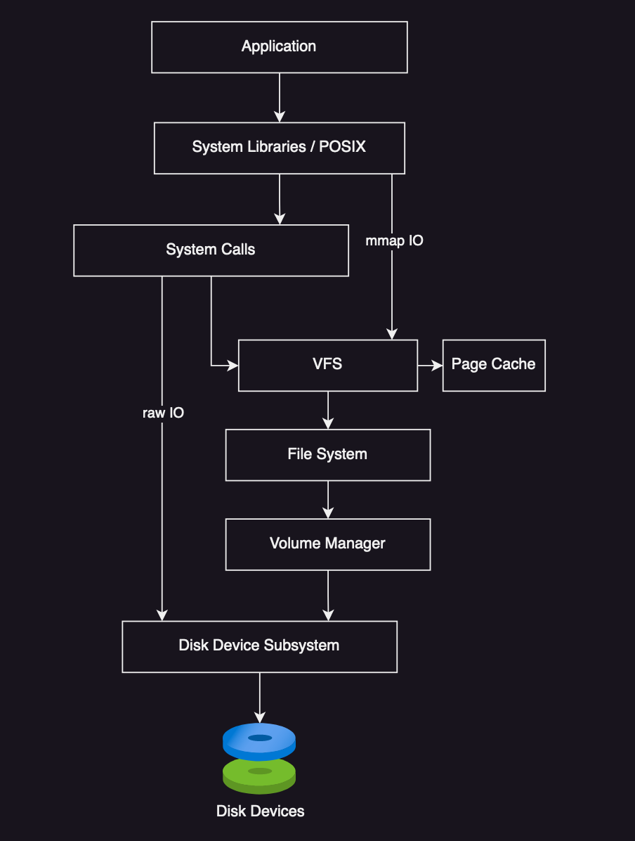
VFS (virtual file system) common interface for different file system types.
File System Caches
Buffer Cache
Page Cache
Dentry Cache
Inode Cache
File System Features
Block (fixed-size) vs Extent (pre-allocated contiguous space)
Journaling
Copy-On-Write
Scrubbing
File System Types
FFS – Berkley fast file system
ext3/ext4
XFS
ZFS
Volume and Pools
Methodology
This section describes various methodologies for file system analysis and tuning:
Disk Analysis
Latency Analysis
Transaction Cost
Workload Characterization
cache hit ratio
cache capacity and utilization
distribution of I/O arrival times
errors
Performance monitoring (operation rate and latency)
Static Performance Tuning
Cache Tuning
Workload Separation
Micro-Benchmaking
Operation types (read/write)
I/O size
File offset pattern
Write type
Working set size
Concurency
Memory mapping
Cache state
Tuning
Observability Tools
mount
free
vmstat
sar
slabtop, e.g.,
slabtop -astrace, e.g.,
strace -ttT -p 123fatrace
opensnoop, e.g.,
opensnoop -Tfiletop
cachestat, e.g.,
cachestat -T 1bpftrace
9. Disks
This chapter provides basis for disk I/O analysis. The parts are as follows:
Models
Simple Disk: includes an on-disk queue for I/O requests
Caching Disk: on-disk cache
Controller: HBA (host-bus adapter) bridges CPU I/O transport with the storage transport and attached disk devices.
Concepts
Measuring Time: I/O request time = I/O wait-time + I/O service-time
disk service time = utilization / IOPS
Time Scales
Caching
Random vs Sequential I/O
Read/Write Ratio
I/O size
Utilization
Saturation
I/O Wait
Synchronous vs Asynchronous
Disk vs Application I/O
Architecture
Disk Types
Magnetic Rotational
max throughput = max sector per track x sector-size x rpm / 60 s
Short-Stroking
Sector Zoning
On-Disk Cache
Solid-State Drives
Flash Memory
Persistent Memory
Interfaces
SCSI
SAS
SATA
NVMe
Storage Type
Disk Devices
RAID
Operating System Disk I/O Stack
Methodology
Tools Method
iostat
iotop/biotop
biolatency
biosnoop
USE Method
Performance Monitoring
Workload Characterization
I/O rate
I/O throughput
I/O size
Read/write ratio
Random vs sequential
Latency Analysis
Static Performance Tuning
Cache Tuning
Micro-Benchmarking
Scaling
Observability Tools
iostat
pressure stall information (PSI)
perf
biolatency, e.g.,
biolatency 10 1biosnoop
biotop
ioping
10. Network
This chapter introduces network analysis. The parts are as follows:
Models
Network Interface
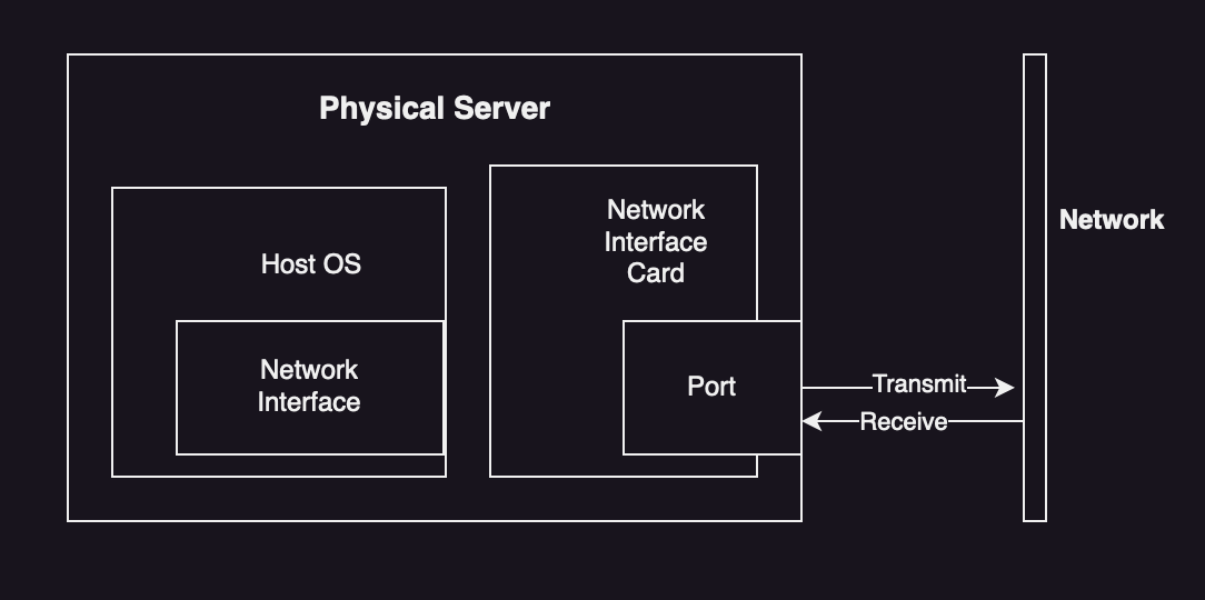
Controller
Protocol Stack
TCP/IP
OSI Model
Concepts
Network and Routing
Protocols
Encapsulation
Packet Size
Latency
Connection Latency
First-Byte Latency
Round-Trip Time
Buffering
Connection Backlog
Congestion Avoidance
Utilization
Local Connection
Architecture
Protocols
IP
TCP
Sliding Window
Congestion avoidance
TCP SYN cookies
3-way Handshake
Duplicate Ack Detection
Congestion Controls
Nagle algorithm
Delayed Acks
UDP
QUIC and HTTP/3
Hardware
Interfaces
Controller
Switches and Routers
Firewalls
Software
Network Stack
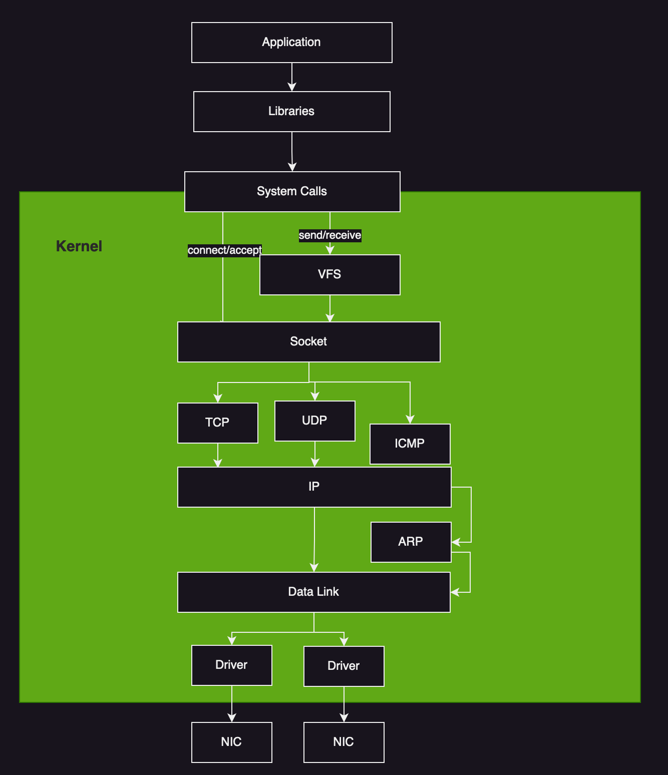
Linux Stack
TCP Connection queues
TCP Buffering
Segmentation Offload: GSO and TSO
Network Device Drivers
CPU Scaling
Kernel Bypass
Methodology
Tools Method
netstat -s
ip -s link
ss -tiepm
nicstat
tcplife
tcptop
tcpdump
USE Method
Workload Characterization
Network interface throughput
Network interface IOPS
TCP connection rate
Latency Analysis
Performance Monitoring
Throughput
Connections
Errors
TCP retransmits
TCP out-of-order pack
Packet Sniffing
tcpdump -ni eth4
TCP Analysis
Static Performance Tuning
Resource Controls
Micro-Benchmarking
Observability Tools
ss, e.g.,
ss -tiepmstrace, e.g.,
strace -e sendmesg,recvmsg ss -tip, e.g.,
ip -s linkifconfig
netstat
sar
nicstat
ethtool, e.g.,
ethtool -S eth0tcplife, tcptop
tcpretrans
bpftrace
tcpdump
wireshark
pathchar
iperf
netperf
tc
Tuning
sysctl -a | grep tcp11. Cloud Computing
This chapter introduces cloud performance analysis with following parts:
Background
Instance Types: m5 (general-purpose), c5 (compute optimized)
Scalable Architecture: horizontal scalability with load balancers, web servers, application servers, and databases.
Capacity Planning: Dynamic sizing (auto-scaling) using auto-scaling-group and and Scalability testing.
Storage: File store, block store, object store
Multitenancy
Orchestration (Kubernetes)
Hardware Virtualization
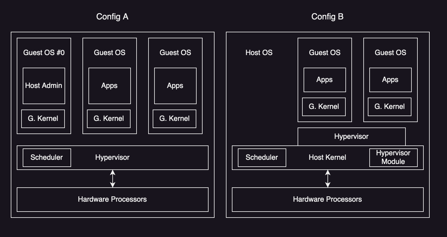
Type 1: execute directly on the processors using native hypervisor or bare-metal hypervisor (e.g., Xen)
Type 2: execute within a host OS and hypervisor is scheduled by the host kernel
Implementation: Xen, Hyper-V, KVM, Nitro
Overhead:
CPU overhead (binary translation, paravirtualization, hardware assisted)
Memory Mapping
Memory Size
I/O
MultiTenant Contention
Resource Controls
Resource Controls
CPUs – Borrowed virtual time, Simple earliest deadline, Credit based schedulers
CPU Caches
Memory Capacity
File System Capacity
Device I/O
Observability
xentop
perf kvm stat live
bpftrace -lv t:kvm:kvm_exit
mpstat -P ALL 1
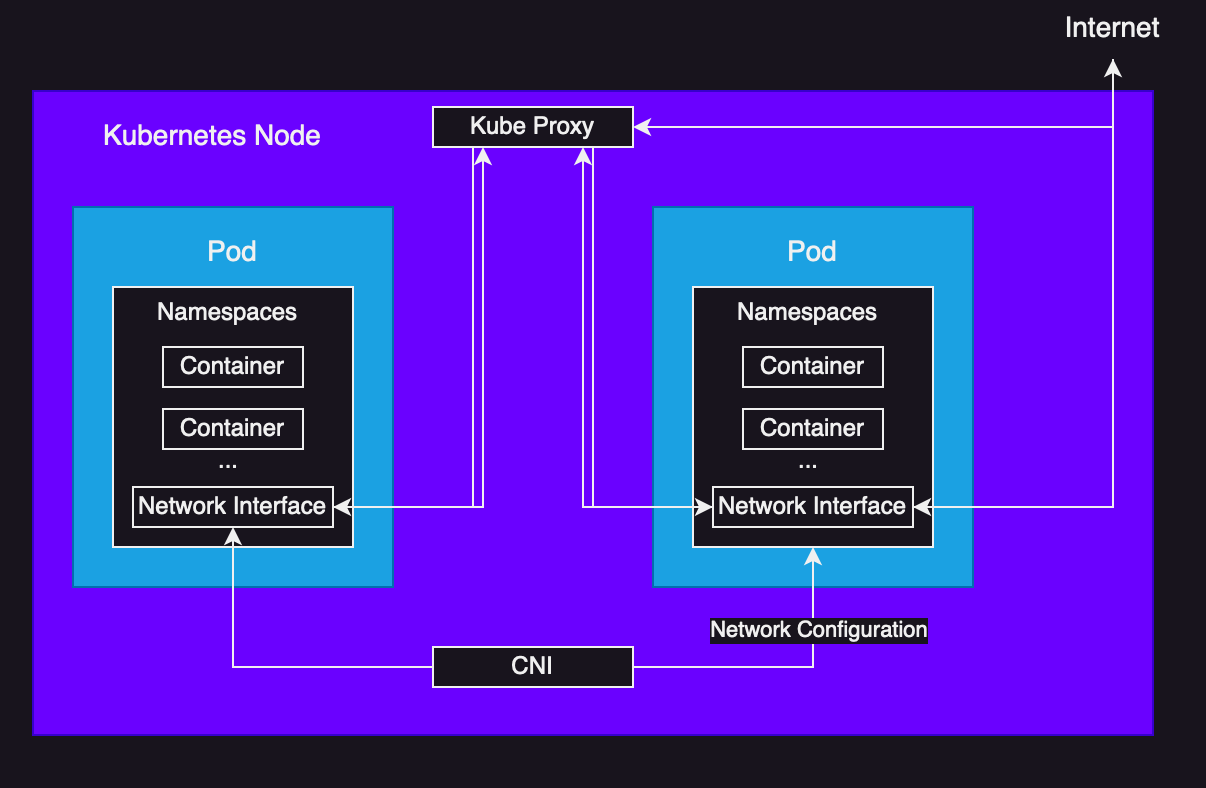
OS Virtualization
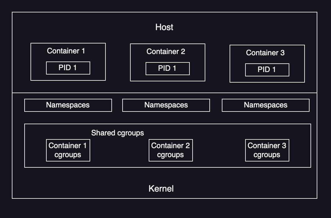
Implementation: Linux supports namespaces and cgroups that are used to create containers. Kubernetes uses following architecture for Pods, Kube Proxy and CNI.
Namespaces
lsns
Control Groups (cgroups) limit the usage of resources
Overhead – CPU, Memory Mapping, Memory Sie, I/O, and Multi-Tenant Contention
Resource Controls – throttle access to resources so they can be shared more fairly
CPU
Shares and Bandwidth
CPU Cache
Memory Capacity
Swap Capacity
File System Capacity
File System Cache
Disk I/O
Network I/O
Observability
from Host
kubectl get pod
docker ps
kubectl top nodes
kubectl top pods
docke stats
cgroup stats (cpuacct.usage and cpuacct.usage_percpu)
system-cgtop
nsenter -t 123 -m -p top
Resource Controls (throttled time, non-voluntary context switches, idle CPU, busy, all other tenants idle)
from guest (container)
iostat -sxz 1
Lightweight Virtualization
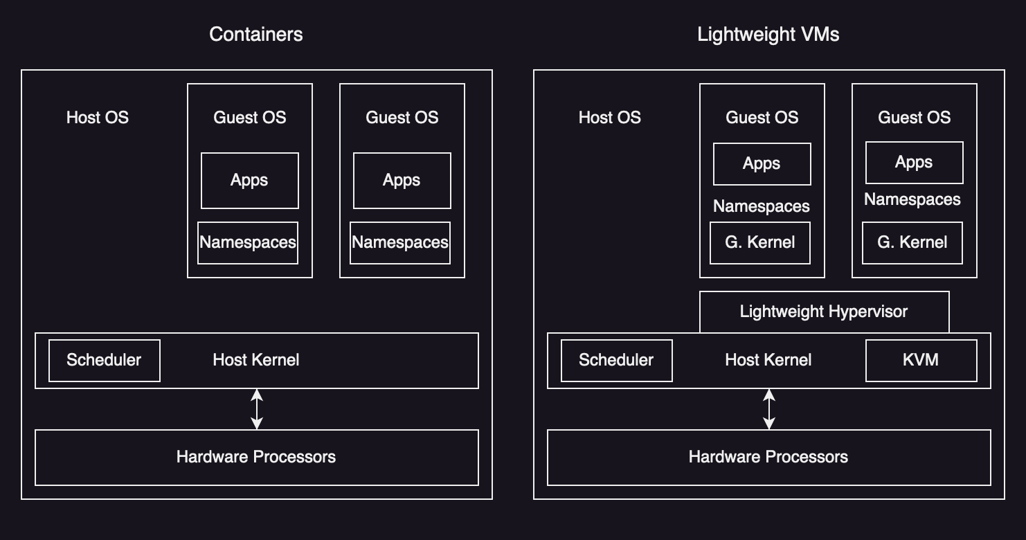
Lightweight hypervisor based on process virtualization (Amazon Firecracker)
Implementation – Intel Clear, Kata, Google gVisor, Amazon Firecracker
Overhead
Resource Controls
Observability
From Host
From Guest
mpstat -P ALL 1
12. Benchmarking
This chapter discusses benchmarks and provides advice with methodologies. The parts of this chapter include:
Background
Reasons
System design
Proof of concept
Tuning
Development
Capacity planning
Troubleshooting
Marketing
Effective Bencharmking
Repeatable
Observable
Portable
Easily presented
Realistic
Runnable
Bencharmk Analysis
Bencharm Failures
Causal Bencharmking – you benchmark A, but measure B, and conclude you measured C, e.g. disk vs file system (buffering/caching may affect measurements).
Blind Faith
Numbers without Analysis – include description of the benchmark and analysis.
Complex Benchmark Tools
Testing the wrong thing
Ignoring the Environment (not tuning same as production)
Ignoring Errors
Ignoring Variance
Ignoring Perturbations
Changing Multiple Factors
Friendly Fire
Benchmarking Types
Micro-Benchmarking
Simulation – simulate customer application workload (macro-bencharmking)
Replay
Industry Standards – TPC, SPEC
Methodology
This section describes methologies for performing becharmking:
Passive Bencharmking (anti-methodology)
pick a BM tool
run with a variety of options
Make a slide of results and share it with management
Problems
Invalid due to software bugs
Limited by benchmark software (e.g., single thread)
Limited by a component that is unrelated to the benchmark (congested network)
Limited by configuration
Subject to perturbation
Benchmarking the wrong the thing entirely
Active Benchmarking
Analyze performance while benchmarking is running
bonie++
iostat -sxz 1
CPU Profiling
USE Method
Workload Characterization
Custom Benchmarks
Ramping Load
Statistical Analysis
Selection of benchmark tool, its configuration
Execution of the benchmark
Interpretation of the data
Benchmarking Checklist
Why not double
Did it beak limit
Did it error
Did it reproduce
Does it matter
Did it even happen
13. perf
This chapter introduces perf tool:
Subcommands Overview
perf record -F 99 -a -- sleep 30
perf Events
perf list
Hardware Events (PMCs)
Frequency Sampling
perf record -vve cycles -a sleep 1
Software Events
perf record -vve context-switches -a -- sleep
Tracepoint Events
perf record -e block:block_rq_issue -a sleep 10; perf script
Probe Events
kprobes, e.g.,
perf prob --add do_nanosleepuprobes, e.g.,
perf probe -x /lib.so.6 --add fopenUSDT
perf stat
Interval Statistics
Per-CPU Balance
Event Filters
Shadow Statistics
perf record
CPU Profiling, e.g.,
perf record -F 99 -a -g -- sleep 30Stack Walking
perf report
TUI
STDIO
perf script
Flame graphs
perf trac
12. Ftrace
This chapter introduces Ftrace tool. The sections are:
Capabilities
tracefs
tracefs contents, e.g.,
ls -F /sys/kernel/debug/tracing
Ftrace Function Profiler
Ftrace Function Tracing
Tracepoints
Filter
Trigger
kprobes
Event Tracing
Argument and Return Values
Filters and Triggers
uprobes
Event Tracing
Argument and Return Values
Ftrace function_graph
Ftrace hwlat
Ftrace Hist Triggers
perf ftrace
15. BPF
This chapter introduces BPF tool. The sections are:
BCC – BPF COmpiler Collection, e.g.,
biolatency.py -mFbpftrace – open-source tracer bult upon BPF and BC
Programming
16. Case Study
This chapter describes the story of a real-world performance issue.
Problem Statement – Java application in AWS EC2 Cloud
Analysis Strategy
Checklist
USE method
Statistics
uptimempstat 10
Configuration
cat /proc/cpuinfo
PMCs
./pmarch -p 123 10
Software Events
perf stat -e cs -a -I 1000
Tracing
cpudist -p 123 10 1
Conclusion
No container neighbors
LLC size and workload diffeence
CPU difference